
See http://www.wenzeltech.com for an
infrasound experiment that captures the sound from the launches of SpaceX
rockets in south Texas (about 300 miles from Austin).
Ft tester
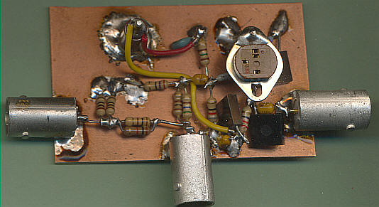
I built a similar Ft tester in the past but this one is pretty simple to use. The test is done at about 10 mA. The CAL and OUT points would typically connect to a scope, preferably through coax terminated with 50 ohms at the scope, but 50 ohm resistors and scope probes should work, too. Other measurement devices will also work. The user plugs in the transistor and adjusts the frequency of the signal generator (set near 10 dBm out or lower) until the signals at CAL and OUT are equal in amplitude. Ft is 20 times that frequency. The DC current can be changed by changing the emitter resistor but lower current will require a smaller test signal. Biased as shown with the 100 ohm emitter resistor 10 dBm is about as big a signal that most transistors can handle without significant distortion. There's no reason to not use a lower amplitude signal if your test equipment can easily observe the smaller signals at the test points.
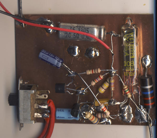
I've now built it (photo below) and it works great! Testing at 1/20th the frequency of Ft makes the layout less critical than one might think. I've successfully tested a 1.5 GHz leaded transistor since the frequency where the two signals are the same size is only 75 MHz (75 x 20 = 1.5 GHz); the test isn't being done at 1.5 GHz. The current gain rises at 20 dB per decade as the frequency decreases and that factor of 20 just manages to keep the measurement on that predictable slope; the signal on the OUT port will begin to flatten with frequency much below that frequency. (Run the LTSpice simulation to see what I mean.)
My 1uF caps have 0.1uF caps in parallel - not a bad idea since low ESR will help the accuracy. 1uF allows the tester to work on the slower transistors.
Here's the LTSpice file with a 2N3904. To see the circuit work, select AC Analysis and run the program. Click on the 1k and collector of the transistor to see those currents (look for the current meter symbol before clicking - looks like a beetle to me : ). The currents intersect at Ft and the collector current rises linearly for lower frequency. Note the frequency of the intersection and divide that number by 20 and notice that the slope is still predictable at that lower frequency. Change the frequency of the generator to this lower frequency. Run the Transient analysis and click on the CAL and OUT points to see the two sine waves. They should be close in amplitude and tweaking the generator frequency will make them equal.
Infrasound Bar Graph
In the modern vernacular, "meh." This thing is just a
wind detector. Seeing the spectrum of the infrasound (using a program like
Spectrum Lab) makes all the difference. There might be a special circumstance
where this simple device will detect a distant infrasound source but there's no
way of knowing unless it's an unusually still day. Not much point, I'm afraid.
However, I do like that simple precision rectifier.
On the other hand, don't miss the nifty precision rectifier for slow, tiny
signals. It's quite nice.
I've built a prototype Infrasound detector that drives a simple bar graph. It detects frequencies below about 15 Hz. The top schematic is a low-pass filter with just a little gain. It could be modified to boost the low-frequency end for microphones that roll off below 20 Hz. AC1 is the microphone but the mic's bias resistor isn't shown. (See the Infrasound page for other preamp circuits and how to add that resistor for the mic. power.)
Ignore the 9 volt supply; the final circuit uses a quad op-amp running on 5 volts. The output above is represented by "V2" below.
Below is a simple precision rectifier that uses only one diode and op-amp, thanks to the nice behavior of the TLC27L7 op-amp when pegged to the bottom rail (the second op-amp is just a low-pass filter and buffer). The red trace is the tiny 10 mV test signal (multiplied by 10 on the plot so you can see it) and the violet trace is the op-amp output gracefully swinging from near-zero out to the voltage required to turn on the diode and charge the .22uF capacitor. The green trace is the voltage on the output and is right at 1 volt. The feedback resistors are selected to give this stage a gain of 100 (peak to DC) so the 10 mV peak sine wave comes out at 10 mV x 100 = 1 VDC. It's a nicely-behaved rectifier for slow, tiny AC signals.
My bar graph is a commercial display but it's quite simple inside, just two LM3914s driving 20 LEDs with a circuit right out of the National data book. But a large analog meter might be even nicer. The bar graph does indicate the presence of "extra" infrasound but it's hard to beat Spectrum Lab for actually seeing what's going on. The idea here is to detect thunder for hundreds of miles. It's easy to see thunder on the spectrum so time will tell if the bar graph is equally informative.
There's little to no wind right now and there's a storm about 400 miles away. Here's what the display looks like. I think that's distant thunder, looking at Spectrum Lab, but there is nearby construction, too. Later - The wind has now picked up (the next day) and wind produces full-scale readings on the bar graph and Spectrum Lab is "lit up" below 10 Hz. These simple infrasound experiments are for calm days! Think of it as an extra "sense" that sometimes means wind and other times it means distant sound sources. When the spectrum lights up with a fairly uniform signal below 15 Hz it's probably a distant storm. Bright lines extending up the frequency scale are usually a close storm or wind, and anything with a pattern of harmonics is probably construction equipment or other man-made source.
I've calculated a new temperature conversion chart for Fenwal 10k, Curve 16 precision thermistors with a Fahrenheit conversion and 0.1C steps. Also see Fenwal 10k thermistors
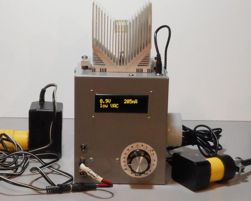
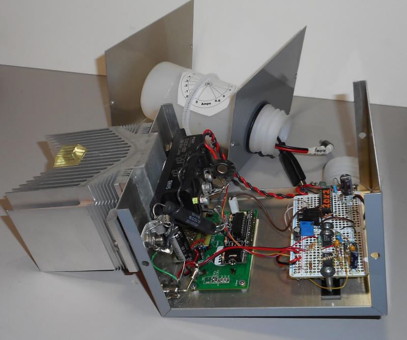
This tester is designed to test various power adapters all the way up to high-power laptop supplies. The heat sink and power transistor are simply overkill! (But it looks great!) The photo on the left shows a 9 volt supply supplying 200 mA (set by dial). The VAC is "low" meaning there's little ripple. There's a polarity-reversing adapter cable plugged in since the supply under test has a negative center pin. The power adapter on the right powers the tester. The inside view reveals the ridiculously overkill power transistor (1/2 of a dual transistor rated at 50 amps and 220 volts!) I'd recommend a more modest power darlington rated at over 5 amps and the heat sink can be much smaller since the tester only runs for a short time. Directly below the black power transistor is the display board from PicAxe.com. To the right are two protoboards from Adafruit, one with a 20X2 Picaxe and the other for the simple analog circuitry. The bottom of the case has a plastic accessory storage bottle held in place by an o-ring. A few adapters are sticking out. There are two jacks on the front for the most common connectors. The circuit is a simple current sink and an audio amplifier/detector for the ripple detection. The circuit is an adjustable current sink with a PicAXE monitoring the noise voltage and actual current.
The schematic doesn't show how the 20X2 connects to the display but that's covered in the PicAXE instructions - quite simple - just connect pin 16 from the 20X2 to the serial input on the display. Here's the PicAXE program. You don't need to know how to program the thing; just paste this program into the PicAXE editor and click on "program." I have a "calibrate frequency" value in mine since the display and 20X2 were having a bit of trouble communicating until I adjusted the frequency a bit. You should probably start with that line removed.
I've made modifications to the King-Sized Infrasound Microphone and the Infrasonic Converter. I've also added the output from these two projects to Live Data.
Here's a silly experiment that's an attempt to find additional uses for the 5886 electrometer tube (typically scrounged from old radiation survey meters). I wanted to see if the tubes could make reasonable front-ends for very high impedance audio amplifiers. My first attempt was a simple grounded-cathode amp and the plate linearity and bandwidth were awful leading me to believe these old tubes might only be good for "D.C." But then I tried a one-transistor feedback amplifier and the circuit came to life. Below are two versions with an added emitter-follower. They perform equally well. The top one is DC-coupled but it does rely on the plate voltage being correct for biasing the rest of the circuit. I'd go with the second circuit in most cases.
The feedback holds the plate voltage fairly constant and the resulting linearity and bandwidth are quite good. I didn't measure the distortion but a sine wave looks great whereas previously it looked like a full-wave rectified sine. The bandwidth is a surprising 400 kHz. The circuit seems to perform just about identically to the same circuit with the tube replaced by an electrometer JFET (like the 2N4117). So why not just use a 2N4117? I only have emotional answers to that question. : ) I suppose this circuit is a bit more immune to static discharge. The input impedance is "crazy high" even without bootstrapping but then it's not exactly low with the FET. If I continue I'm grasping at straws.
Note how little current the filament needs; it's not much more than a typical transistor stage.
I used a 22 megohm to ground the gate but that could just as well be a 100 gigohm or even a neon lamp with its internal radioactive isotope.
I moved the solar flare stuff to: Solar Flare Project